Correction playground#

This serves as an example on how an analyst can modify/add corrections according to their analysis. It builds on the SysVar 101 example so it is consistent and easy to follow. We will demonstrate here PID, BF and custom corrections as described in the corrections chapter since these are the ones that are very analysis specific and requires the analyst to describe them accordingly.

[1]:

%reload_ext autoreload
%autoreload 2

BF corrections#

To the same toy_df, now we added another column called dmID. This essentially categorizes the signal into two decays marked by 11 and 12 and bkg by 21. This information is required for the BF corrections to be able to reweight the event.

[3]:

toy_df

[3]:

	channel	template	slow_pi_p	slow_pi_mcPDG	slow_pi_PDG	fit_variable1	fit_variable2	other_weight	slow_pi_dmID
0	1	signal	0.180663	-211	-211	0.116426	2.256413	0.361459	11
1	1	signal	0.206703	211	-211	0.157742	2.124415	0.392474	11
2	1	signal	0.088177	211	-211	0.172442	2.822007	0.255194	11
3	0	signal	0.113488	-211	-211	0.802428	3.060842	0.238842	12
4	0	signal	0.091468	-211	-211	0.205307	1.932665	0.363094	11
...	...	...	...	...	...	...	...	...	...
1995	1	signal	0.135897	-211	-211	0.038330	2.596879	0.258352	12
1996	1	signal	0.120251	-211	211	0.032259	2.380286	0.330346	12
1997	1	bkg	0.130750	211	-211	0.849735	3.960611	0.803959	21
1998	0	signal	0.225188	211	211	0.236084	2.295463	0.335913	12
1999	1	signal	0.216735	211	211	0.119552	2.515693	0.297056	12

1760 rows × 9 columns

Suppose, by default the MC signal events were generated with BF of 55% for decay 11 and 45% for decay 12. Now, there is some new information available on them after the generation that this should rather be 53% and 47% with uncertainties on the measurement also provided.

We can add these weights to the dataframe by setting up a config file as follows. The important attributes are:

dependant_variable: Variable in your dataframe which categorizes the decay.
mother_particle: For visualization purposes, PDG ID of the mother particle in decay chain.
modes:
- name of the decay: For visualization, you can name the decay
- daughters: A list of the daughter particle PDG IDs for visualization
- pdg_live: A list where first column is the new measurement weight and second column the uncertainty.
- decay_dec: Original weight with which the event was generated.

[4]:

from sysvar.utils import read_yaml

BF_config = read_yaml("BF_101", "sysvar_101")
BF_config

[4]:

{'correction_type': 'BF',
 'correlation': 'uncorrelated',
 'dependant_variable': 'dmID',
 'mother_particle': 211,
 'title': 'SysVar 101 Branching fraction',
 'extra_cuts': None,
 'modes': {'Signal_decay_1': {'dmID': [11],
   'daughters': [[211]],
   'pdg_live': [0.53, 0.01],
   'decay_dec': 0.55},
  'Signal_decay_2': {'dmID': [12],
   'daughters': [[211]],
   'pdg_live': [0.47, 0.011],
   'decay_dec': 0.45}}}

[5]:

from sysvar import add_weights_to_dataframe

add_weights_to_dataframe(
    df = toy_df,
    systematic= "BF_101",
    MC_production= "sysvar_101",
    prefix= "slow_pi",
    weightname ="BF_weight",
    #overwrite: False,
    Nvar =  2
)
toy_df

WARNING : load_covariance_matrix: 190 :  Explicit covariance matrix was not found in config under None or cov_matrix_path and will be built from the specified uncertainties.
INFO : add_weights_to_dataframe: 103 :  slow_pi_BF_weight does not exist. Adding it to dataframe

[5]:

	channel	template	slow_pi_p	slow_pi_mcPDG	slow_pi_PDG	fit_variable1	fit_variable2	other_weight	slow_pi_dmID	slow_pi_BF_weight	slow_pi_BF_weight_var_0	slow_pi_BF_weight_var_1
0	1	signal	0.180663	-211	-211	0.116426	2.256413	0.361459	11	0.963636	0.945115	0.961559
1	1	signal	0.206703	211	-211	0.157742	2.124415	0.392474	11	0.963636	0.945115	0.961559
2	1	signal	0.088177	211	-211	0.172442	2.822007	0.255194	11	0.963636	0.945115	0.961559
3	0	signal	0.113488	-211	-211	0.802428	3.060842	0.238842	12	1.044444	1.079652	1.102055
4	0	signal	0.091468	-211	-211	0.205307	1.932665	0.363094	11	0.963636	0.945115	0.961559
...	...	...	...	...	...	...	...	...	...	...	...	...
1995	1	signal	0.135897	-211	-211	0.038330	2.596879	0.258352	12	1.044444	1.079652	1.102055
1996	1	signal	0.120251	-211	211	0.032259	2.380286	0.330346	12	1.044444	1.079652	1.102055
1997	1	bkg	0.130750	211	-211	0.849735	3.960611	0.803959	21	1.000000	1.000000	1.000000
1998	0	signal	0.225188	211	211	0.236084	2.295463	0.335913	12	1.044444	1.079652	1.102055
1999	1	signal	0.216735	211	211	0.119552	2.515693	0.297056	12	1.044444	1.079652	1.102055

1760 rows × 12 columns

PID corrections#

PID corrections are also analysis specific and the tables should be generated using the systematics framework with the selection cuts of your analysis. This table can be specified in the config file as follows. The dataframe should information on momentum p, angle theta, reconstructed PDG ID PDG and generated PDG ID mcPDG

[6]:

PID_config = read_yaml("PID_101", "sysvar_101")
PID_config

[6]:

{'correction_type': 'PID',
 'rate': 'eff',
 'momentum_unit': 'GeV',
 'title': 'SysVar 101 PID corrections',
 'momentum_variable': 'p',
 'theta_variable': 'theta',
 'PDG_variable': 'PDG',
 'mcPDG_variable': 'mcPDG',
 'extra_cuts': None,
 'online_cut': 'PIDcut > x.y',
 'table_paths': '/path/to/your/table/generated/using/systematicsframework/'}

Custom Correction#

Let’s first assume that you perform a calibration specific to your analysis. In this example, suppose you have performed a fit in a control region (CR) to extract correction weights that depend on the charge of the slow pion, determined separately for signal and background.

Let’s add this info into the dataframe

[7]:

toy_df["custom_calibration_id"] = "0"
toy_df["custom_calibration_weight"] = 1.0

mask = (toy_df["template"] == "signal") & (toy_df["slow_pi_PDG"] == -211)
toy_df.loc[mask , "custom_calibration_id"] = "-10211"
toy_df.loc[mask, "custom_calibration_weight"] = 1.0115


mask = (toy_df["template"] == "signal") & (toy_df["slow_pi_PDG"] == 211)
toy_df.loc[mask , "custom_calibration_id"] = "10211"
toy_df.loc[mask, "custom_calibration_weight"] = 0.8532

mask = (toy_df["template"] == "bkg") & (toy_df["slow_pi_PDG"] == -211)
toy_df.loc[mask , "custom_calibration_id"] = "-20211"
toy_df.loc[mask, "custom_calibration_weight"] = 1.1194


mask = (toy_df["template"] == "bkg") & (toy_df["slow_pi_PDG"] == 211)
toy_df.loc[mask , "custom_calibration_id"] = "20211"
toy_df.loc[mask, "custom_calibration_weight"] = 0.9663

toy_df["total_weight"] = toy_df[["other_weight", "custom_calibration_weight"]].product(axis = 1)

At the moment, SysVar does not natively support adding custom corrections directly to the dataframe, unless you manually create a dedicated YAML or CSV file. For this example, we will assume that the custom correction is already present in the dataframe.

Now let’s create the dictionary that SysVar expects when building custom corrections:

[8]:

custom_calibration_info = {
    'dependant_variable': 'custom_calibration_id',
     'central_values': [1.0115, 0.8532, 1.1194, 0.9663,
      ],
     'query_targets': ["-10211", "10211", "-20211", "20211"], # These have to be strings
     'uncertainties': {'uncorrelated': {'unc': [0.0528, 0.0926, 0.1766, 0.0942]}},
     'unit': '',
     'title': 'custom_calibration_weight',
     'name': 'custom_calibration'}

Now, in the eigendecompose call, instead of passing the name of the systematic set, you should pass the custom calibration information, e.g. systematic_effect = custom_calibration_info

Before calling eigendecompose however, you need to update the main configuration file so that SysVar knows which templates and which channels are affected by this systematic.

[9]:

from sysvar.utils import read_yaml

settings = read_yaml("study_setup", "sysvar_101")

[10]:

settings["systematics"]["custom_calibration"] = {
    'weight': 'custom_calibration_weight',
    'prefices': [],
    'reco_channels': {'include': None, 'exclude': None},
    "templates": ["bkg", "signal"],
}

Now let’s run eigedecompose

[11]:

from sysvar import eigendecompose

egd_custom = eigendecompose(
    df = toy_df,
    settings = settings,
    syst_effect = custom_calibration_info, # Notice that instead of a string here we pass a dictionary
)

WARNING : load_covariance_matrix: 190 :  Explicit covariance matrix was not found in config under None or cov_matrix_path and will be built from the specified uncertainties.
/Users/agrimaggarwal/Documents/PhD/frameworks/sysvar/src/sysvar/variations.py:143: RuntimeWarning: divide by zero encountered in matmul
  return rng.multivariate_normal(zeros, covariance, Nvar)
/Users/agrimaggarwal/Documents/PhD/frameworks/sysvar/src/sysvar/variations.py:143: RuntimeWarning: overflow encountered in matmul
  return rng.multivariate_normal(zeros, covariance, Nvar)
/Users/agrimaggarwal/Documents/PhD/frameworks/sysvar/src/sysvar/variations.py:143: RuntimeWarning: invalid value encountered in matmul
  return rng.multivariate_normal(zeros, covariance, Nvar)
INFO : create_templates: 184 :  ########## Reco channel: channel1 ##########
INFO : create_templates: 215 :  Building TemplateND for bkg from 378 events
INFO : create_templates: 215 :  Building TemplateND for signal from 474 events
INFO : create_templates: 184 :  ########## Reco channel: channel2 ##########
INFO : create_templates: 215 :  Building TemplateND for bkg from 385 events
INFO : create_templates: 215 :  Building TemplateND for signal from 519 events
INFO : vary_templates: 162 :  ########## Reco channel: channel1 ##########
INFO : vary_templates: 176 :  Adding variations to bkg template
INFO : vary_templates: 176 :  Adding variations to signal template
INFO : vary_templates: 162 :  ########## Reco channel: channel2 ##########
INFO : vary_templates: 176 :  Adding variations to bkg template
INFO : vary_templates: 176 :  Adding variations to signal template
WARNING : max_differences: 131 :  Only the first 60 eigendirections will be considered to find the maximum number of eigenvariations.
Building partial covariances: 100%|██████████| 60/60 [00:00<00:00, 12792.71it/s]
INFO : find_important_eigendimension_indices: 202 :  Found that 4 eigendirections matter for 0.0001 per cent precision

Let’s check how many eigenvariations we’re saving.

[12]:

from sysvar import plot_cov_diff

fig, ax = plot_cov_diff(egd_custom)

../_images/notebooks_correction_playground_24_0.png

This is consistent with what we mentioned earlier in the Information for Analysts: we retain the 4 dominant eigendirections, since there are only 4 uncorrelated correction weights.

What would happen if the errors were fully correlated ?

[13]:

custom_calibration_info = {
    'dependant_variable': 'custom_calibration_id',
     'central_values': [1.0115, 0.8532, 1.1194, 0.9663,
      ],
     'query_targets': ["-10211", "10211", "-20211", "20211"], # These have to be strings
     'uncertainties': {'fully_correlated': {'unc': [0.0528, 0.0926, 0.1766, 0.0942]}},
     'unit': '',
     'title': 'custom_calibration_weight',
     'name': 'custom_calibration'}

[14]:

egd_custom_fully_corr = eigendecompose(
    df = toy_df,
    settings = settings,
    syst_effect = custom_calibration_info, # Notice that instead of a string here we pass a dictionary
)
fig, ax = plot_cov_diff(egd_custom_fully_corr)

WARNING : load_covariance_matrix: 190 :  Explicit covariance matrix was not found in config under None or cov_matrix_path and will be built from the specified uncertainties.
/Users/agrimaggarwal/Documents/PhD/frameworks/sysvar/src/sysvar/variations.py:143: RuntimeWarning: divide by zero encountered in matmul
  return rng.multivariate_normal(zeros, covariance, Nvar)
/Users/agrimaggarwal/Documents/PhD/frameworks/sysvar/src/sysvar/variations.py:143: RuntimeWarning: overflow encountered in matmul
  return rng.multivariate_normal(zeros, covariance, Nvar)
/Users/agrimaggarwal/Documents/PhD/frameworks/sysvar/src/sysvar/variations.py:143: RuntimeWarning: invalid value encountered in matmul
  return rng.multivariate_normal(zeros, covariance, Nvar)
INFO : create_templates: 184 :  ########## Reco channel: channel1 ##########
INFO : create_templates: 215 :  Building TemplateND for bkg from 378 events
INFO : create_templates: 215 :  Building TemplateND for signal from 474 events
INFO : create_templates: 184 :  ########## Reco channel: channel2 ##########
INFO : create_templates: 215 :  Building TemplateND for bkg from 385 events
INFO : create_templates: 215 :  Building TemplateND for signal from 519 events
INFO : vary_templates: 162 :  ########## Reco channel: channel1 ##########
INFO : vary_templates: 176 :  Adding variations to bkg template
INFO : vary_templates: 176 :  Adding variations to signal template
INFO : vary_templates: 162 :  ########## Reco channel: channel2 ##########
INFO : vary_templates: 176 :  Adding variations to bkg template
INFO : vary_templates: 176 :  Adding variations to signal template
WARNING : max_differences: 131 :  Only the first 59 eigendirections will be considered to find the maximum number of eigenvariations.
Building partial covariances: 100%|██████████| 58/58 [00:00<00:00, 14374.24it/s]
INFO : find_important_eigendimension_indices: 202 :  Found that 1 eigendirections matter for 0.0001 per cent precision

../_images/notebooks_correction_playground_27_1.png

Notice that now we retain only one dominant eigendirection, since the errors are fully correlated.

If these correction weights were obtained from a simultaneous fit and the covariance matrix between them is already available, you can pass this matrix directly to the custom_calibration_info dictionary. Now there is no need to specify the individual errors separately.

[16]:

custom_calibration_info = {
    'dependant_variable': 'custom_calibration_id',
     'central_values': [1.0115, 0.8532, 1.1194, 0.9663,
      ],
     'query_targets': ["-10211", "10211", "-20211", "20211"],
     'unit': '',
     'title': 'custom_calibration_weight',
     'name': 'custom_calibration'}

Now we need to specify the covariance matrix path and then run the eigendecomposition

[17]:

custom_calibration_info["cov_matrix_path"] = "cov_custom.npy"

[18]:

egd_custom_partial_corr = eigendecompose(
    df = toy_df,
    settings = settings,
    syst_effect = custom_calibration_info,
)
fig, ax = plot_cov_diff(egd_custom_partial_corr)

INFO : load_covariance_matrix: 182 :  Loading covariance matrix from file specified in config: cov_custom.npy
/Users/agrimaggarwal/Documents/PhD/frameworks/sysvar/src/sysvar/variations.py:143: RuntimeWarning: covariance is not symmetric positive-semidefinite.
  return rng.multivariate_normal(zeros, covariance, Nvar)
/Users/agrimaggarwal/Documents/PhD/frameworks/sysvar/src/sysvar/variations.py:143: RuntimeWarning: divide by zero encountered in matmul
  return rng.multivariate_normal(zeros, covariance, Nvar)
/Users/agrimaggarwal/Documents/PhD/frameworks/sysvar/src/sysvar/variations.py:143: RuntimeWarning: overflow encountered in matmul
  return rng.multivariate_normal(zeros, covariance, Nvar)
/Users/agrimaggarwal/Documents/PhD/frameworks/sysvar/src/sysvar/variations.py:143: RuntimeWarning: invalid value encountered in matmul
  return rng.multivariate_normal(zeros, covariance, Nvar)
INFO : create_templates: 184 :  ########## Reco channel: channel1 ##########
INFO : create_templates: 215 :  Building TemplateND for bkg from 378 events
INFO : create_templates: 215 :  Building TemplateND for signal from 474 events
INFO : create_templates: 184 :  ########## Reco channel: channel2 ##########
INFO : create_templates: 215 :  Building TemplateND for bkg from 385 events
INFO : create_templates: 215 :  Building TemplateND for signal from 519 events
INFO : vary_templates: 162 :  ########## Reco channel: channel1 ##########
INFO : vary_templates: 176 :  Adding variations to bkg template
INFO : vary_templates: 176 :  Adding variations to signal template
INFO : vary_templates: 162 :  ########## Reco channel: channel2 ##########
INFO : vary_templates: 176 :  Adding variations to bkg template
INFO : vary_templates: 176 :  Adding variations to signal template
WARNING : max_differences: 131 :  Only the first 60 eigendirections will be considered to find the maximum number of eigenvariations.
Building partial covariances: 100%|██████████| 60/60 [00:00<00:00, 15079.29it/s]
INFO : find_important_eigendimension_indices: 202 :  Found that 3 eigendirections matter for 0.0001 per cent precision

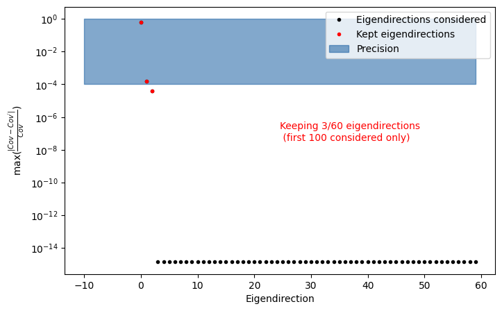
../_images/notebooks_correction_playground_33_1.png

In this case, the number of relevant eigenvariations depends on the off-diagonal terms of the covariance matrix of the corrections. You can inspect the covariance matrix directly via egd_custom_partial_corr.variator.cov_matrix or use the Visualization API (see next section).

Partial correlations are exactly the situations where SysVar’s full machinery provides the greatest advantage—beyond the book-keeping functionality, which remains relevant for the two cases we examined above.

Correction playground

Contents

Correction playground#

BF corrections#

PID corrections#

Custom Correction#