SysVar 101#
The full notebook can be found here
This notebook provides a minimal example on how to use SysVar.#
We will create Eigenvariations of our fitting variable based on the charged slow pion corrections in 2 reconstruction channels and for 2 templates in 15 bins
[1]:
%reload_ext autoreload
%autoreload 2
Attention:#
Setting the SysVar Path#
Please update the path below to point to the location where you have installed your SysVar fork, then execute the cell.
This step is currently necessary because the basf2 developers have renamed their pidvar class to sysvar, anticipating an early merge of the SysVar package into basf2.
If you are running with an environment sourced from CVMFS and have not executed the cell below, you will encounter the following error:
ModuleNotFoundError: No module named 'sysvar.utils'; 'sysvar' is not a package
To avoid this error, set the correct path to your SysVar installation and run the cell.
[2]:
import sys
sys.path.insert(0,'{path_where_you_pip_installed_sysvar}/SysVar/src')
A minimal dataframe#
[4]:
toy_df
[4]:
| channel | template | slow_pi_p | slow_pi_mcPDG | slow_pi_PDG | fit_variable1 | fit_variable2 | other_weight | |
|---|---|---|---|---|---|---|---|---|
| 0 | 1 | bkg | 0.092206 | -211 | -211 | 0.124971 | 1.285126 | 0.777656 |
| 1 | 0 | signal | 0.143104 | -211 | -211 | 0.157658 | 2.671896 | 0.205174 |
| 2 | 1 | signal | 0.142781 | -211 | 211 | 0.228848 | 2.302597 | 0.259262 |
| 3 | 0 | bkg | 0.138268 | 211 | -211 | 0.873285 | 2.648161 | 0.849751 |
| 4 | 1 | signal | 0.111139 | 211 | -211 | 0.020973 | 2.353314 | 0.321819 |
| ... | ... | ... | ... | ... | ... | ... | ... | ... |
| 1995 | 1 | signal | 0.096564 | -211 | -211 | 0.341391 | 2.364311 | 0.282196 |
| 1996 | 1 | signal | 0.186003 | -211 | 211 | 0.148289 | 2.405311 | 0.241490 |
| 1997 | 1 | bkg | 0.115481 | -211 | -211 | 0.710345 | 1.309865 | 0.905345 |
| 1998 | 0 | signal | 0.124871 | -211 | -211 | 0.287474 | 2.577334 | 0.321341 |
| 1999 | 0 | bkg | 0.152832 | 211 | 211 | 0.757065 | 2.512988 | 0.785640 |
1788 rows × 8 columns
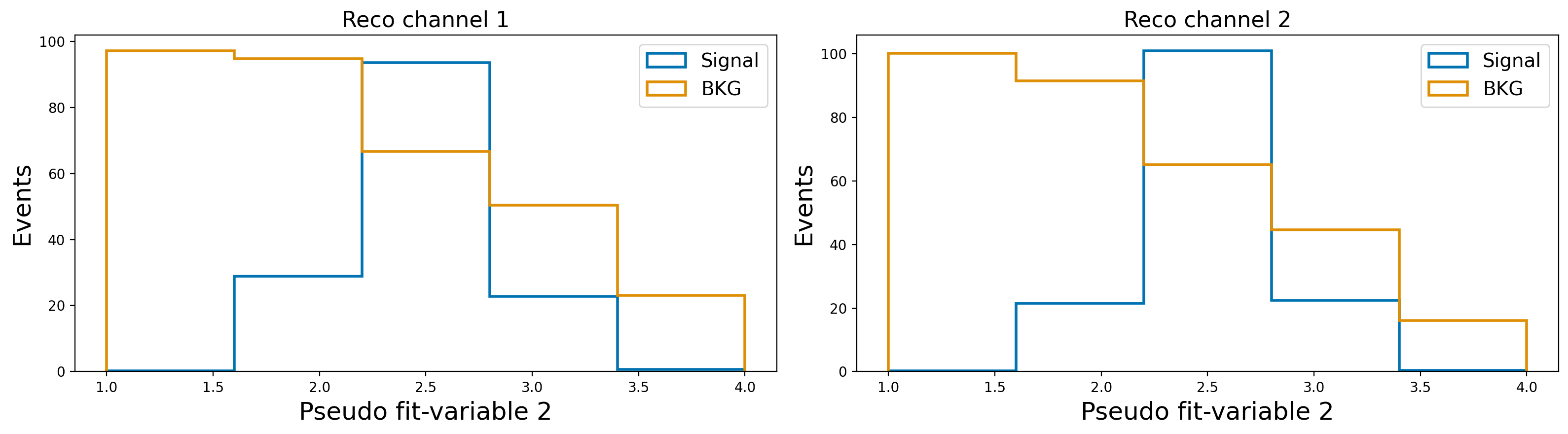
Let’s plot what we have#
[5]:
PALETTE = sns.color_palette("colorblind")


def plot_var_in_2_channels(column_name, xlabel, bins, scope):

    fig, ax = plt.subplots(1, 2, figsize = (16, 4.5), dpi = 200)

    for i, c in enumerate(toy_df.channel.value_counts().keys()):
        for j, t in enumerate(toy_df.template.value_counts().keys()):
            tmp_df = toy_df.query(f"channel == {c} & template == '{t}'")
            ax[i].hist(
                tmp_df[column_name],
                weights=tmp_df["other_weight"],
                histtype = "step",
                label = "Signal" if t == "signal" else "BKG",
                bins = bins,
                range = scope,
                linewidth = 2,
                color = PALETTE[j]
            )
        ax[i].legend(fontsize=14)
        ax[i].set_xlabel(xlabel, fontsize=18)
        ax[i].set_ylabel("Events", fontsize=18)
        ax[i].set_title(f"Reco channel {i+1}", fontsize=16)


plot_var_in_2_channels("fit_variable1", "Pseudo fit-variable 1", bins = 5, scope = (0,1))
plt.tight_layout()
#plt.savefig("pseudofit1.png", dpi = 200)
plot_var_in_2_channels("fit_variable2", "Pseudo fit-variable 2", bins = 5, scope = (1,4))
plt.tight_layout()
#plt.savefig("pseudofit2.png", dpi = 200)
plot_var_in_2_channels("slow_pi_p", r"$p_{\pi_{s}}$ in GeV", bins = [0.05, 0.12, 0.16, 0.2, 0.4], scope = (0, 0.4))
plt.tight_layout()
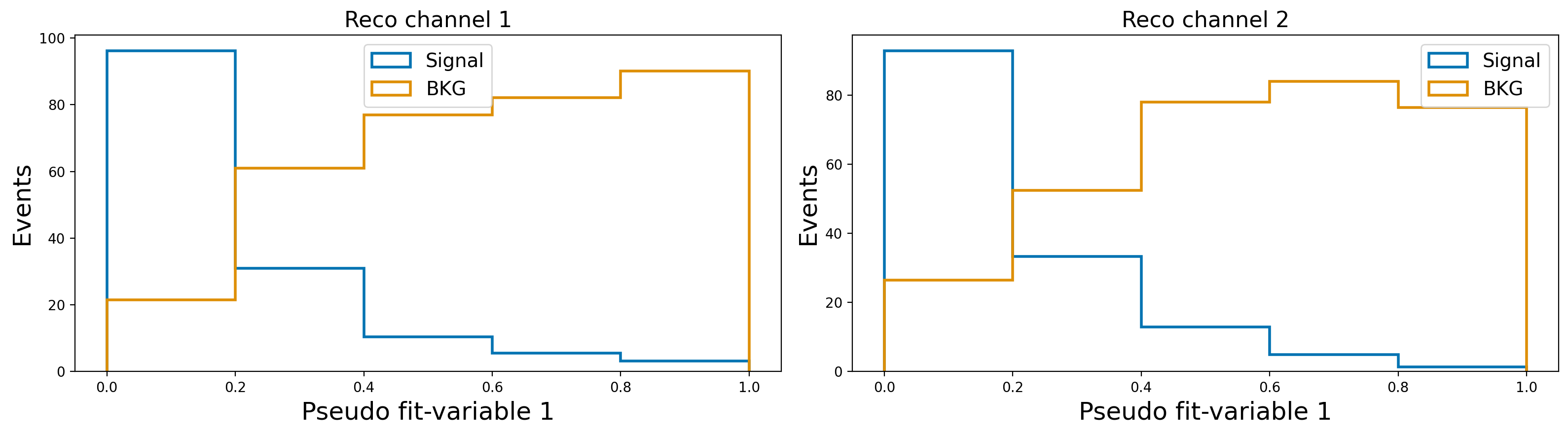
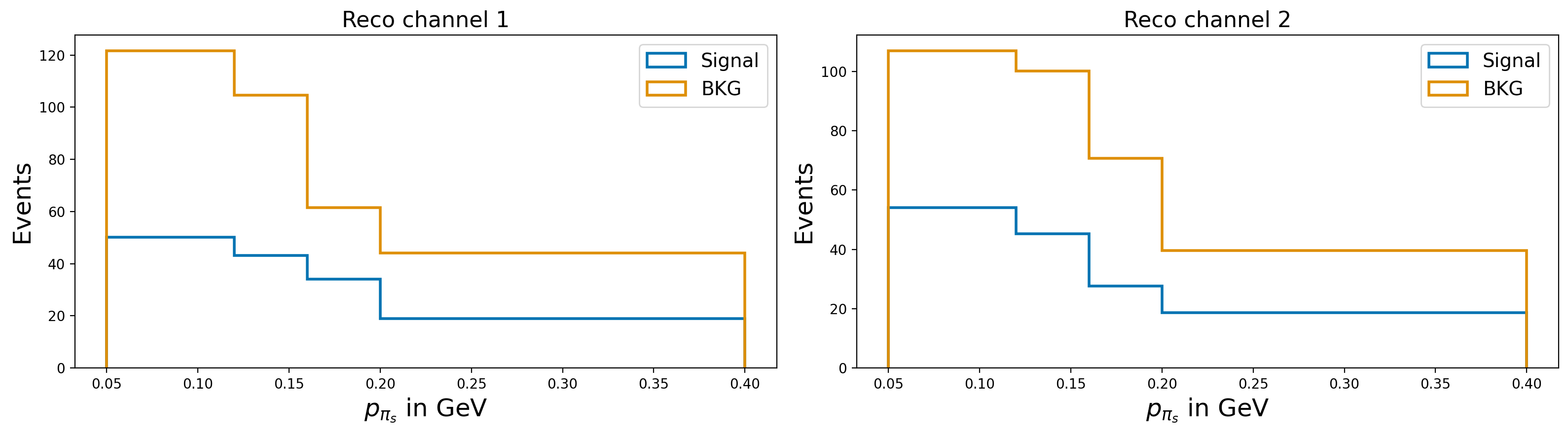
Let’s assume that the slow–pion efficiency differs between MC and data, so we need to correct the MC.
Further assume that this efficiency correction is provided in bins of the slow–pion momentum. These corrections will need to be supplied to SysVar (details follow in the next sections).
For now, we will illustrate the procedure using a pseudo-correction defined in three momentum bins for the slow pion.
These correction weights may be partially correlated across bins, due to both statistical and systematic uncertainties. Events with slow pions in different momentum bins can populate different bins of the signal-extraction observables, and therefore the induced correlation between those templates is not trivial to compute by hand.
Our task is to propagate the correlations from the correction-weight space (momentum bins) to the signal-extraction space (template bins) in a consistent way.
Now let’s add slow pion weights to the dataframe#
Information necessary in the dataframe for charged slow pion: Looking at the config file for charged_slow_pion corrections
dependent variable:
pextra_cuts:
PDG
For Belle II analyses, these are the basf2 variable information required in the dataframe for this correction to work. A prefix can be chosen to distinguish between different particles or also can be provided as a list of prefices. Here a prefix "slow_pi" is provided. This requires the dataframe to contain the variables slow_pi_p, slow_pi_PDG. A weightname for the corresponding correction is required and if a
prefix is provided it will be prepended to that name. In the example, we add a variable called slow_pi_charged_weight.
[6]:
from sysvar import add_weights_to_dataframe

add_weights_to_dataframe(
    df = toy_df,
    systematic= "charged_slow_pi",
    MC_production= "sysvar_101",
    prefix= "slow_pi",
    weightname ="charged_weight",
    #overwrite: False,
    #Nvar: 0
)
toy_df
WARNING : load_covariance_matrix: 190 :  Explicit covariance matrix was not found in config under None or cov_matrix_path and will be built from the specified uncertainties.
INFO : read_corrections: 392 :  Loading correction values from config array.
INFO : add_weights_to_dataframe: 103 :  slow_pi_charged_weight does not exist. Adding it to dataframe
[6]:
| channel | template | slow_pi_p | slow_pi_mcPDG | slow_pi_PDG | fit_variable1 | fit_variable2 | other_weight | slow_pi_charged_weight | |
|---|---|---|---|---|---|---|---|---|---|
| 0 | 1 | bkg | 0.092206 | -211 | -211 | 0.124971 | 1.285126 | 0.777656 | 0.977 |
| 1 | 0 | signal | 0.143104 | -211 | -211 | 0.157658 | 2.671896 | 0.205174 | 0.989 |
| 2 | 1 | signal | 0.142781 | -211 | 211 | 0.228848 | 2.302597 | 0.259262 | 0.989 |
| 3 | 0 | bkg | 0.138268 | 211 | -211 | 0.873285 | 2.648161 | 0.849751 | 0.989 |
| 4 | 1 | signal | 0.111139 | 211 | -211 | 0.020973 | 2.353314 | 0.321819 | 0.977 |
| ... | ... | ... | ... | ... | ... | ... | ... | ... | ... |
| 1995 | 1 | signal | 0.096564 | -211 | -211 | 0.341391 | 2.364311 | 0.282196 | 0.977 |
| 1996 | 1 | signal | 0.186003 | -211 | 211 | 0.148289 | 2.405311 | 0.241490 | 0.943 |
| 1997 | 1 | bkg | 0.115481 | -211 | -211 | 0.710345 | 1.309865 | 0.905345 | 0.977 |
| 1998 | 0 | signal | 0.124871 | -211 | -211 | 0.287474 | 2.577334 | 0.321341 | 0.989 |
| 1999 | 0 | bkg | 0.152832 | 211 | 211 | 0.757065 | 2.512988 | 0.785640 | 0.989 |
1788 rows × 9 columns
If you try again, then SysVar will complain. In order to overwrite an existing weight, set the relevant argument to True
[7]:
add_weights_to_dataframe(
    df = toy_df,
    systematic= "charged_slow_pi",
    MC_production= "sysvar_101",
    prefix= "slow_pi",
    weightname ="charged_weight",
    overwrite= False
)
WARNING : load_covariance_matrix: 190 :  Explicit covariance matrix was not found in config under None or cov_matrix_path and will be built from the specified uncertainties.
INFO : read_corrections: 392 :  Loading correction values from config array.
WARNING : add_weights_to_dataframe: 98 :  slow_pi_charged_weight exists but it not will be ovewritten. Skipping. No weights are added. If you want to change this behaviour set the overwrite argument to True
Now we create the total weight of the analysis
[8]:
toy_df["total_weight"] = toy_df[["other_weight", "slow_pi_charged_weight"]].product(axis = 1)
Define the configurations for the Eigen decomposition#
Instructions for the SysVar Configuration File#
This configuration file is the primary interface for communicating with SysVar. Your entire analysis setup should be encoded here.
Parameters#
output_filepath:The path where both nominal templates and all template variations will be saved. Currently, only root files are supported.reco_channel_id_column:The name of the column in your dataframe that distinguishes different reconstruction channels to be fitted separately but simultaneously.reco_channels:A dictionary mapping custom channel names (as keys) to lists of values to be found in thereco_channel_id_column.template_id_column:The name of the column in your dataframe that distinguishes different templates.templates:A list of template names. These should correspond to values found in thetemplate_id_columnof your dataframe.total_weight:The total weight to use when creating nominal templates for your analysis.MC_prod:The Belle II MC campaign. Currently, onlyMC15rdis supported.Nvar:The number of weight variations to generate.bins:A nested dictionary defining the binning for each channel and variable. Both 1D and ND histogram projections are supported.systematics:A nested dictionary. Each top-level key corresponds to a systematic name. For every systematic entry, the following fields must be provided:There should be a corresponding YAML file in the configs (see configs/MC15rd).
The key
weightshould contain the name of the column with the weight associated with this systematic.prefices: A string or list of strings to prepend to the weight name to build the column name present in the dataframe.reco_channels: Specify a list of channels (as strings) to include or exclude in the systematic variation. If both areNone, all channels will be affected.templates: Specify a list of templates (as strings) to include or exclude in the systematic variation. Defaults toNone(all templates affected).
Below you can see the configuration file that corresponds to this mininal example
[9]:
from sysvar.utils import read_yaml

settings = read_yaml("study_setup_101", "sysvar_101")
settings
[9]:
{'output_filepath': './test_output.root',
 'reco_channel_id_column': 'channel',
 'reco_channels': {'channel1': [0], 'channel2': [1]},
 'template_id_column': 'template',
 'templates': ['signal', 'bkg'],
 'total_weight': 'total_weight',
 'MC_prod': 'sysvar_101',
 'Nvar': 500,
 'bins': {'channel1': {'fit_variable1': [0, 0.2, 0.4, 0.6, 0.8, 1],
   'fit_variable2': [1, 2, 3, 4]},
  'channel2': {'fit_variable1': [0, 0.2, 0.4, 0.6, 0.8, 1],
   'fit_variable2': [1, 2, 3, 4]}},
 'systematics': {'charged_slow_pi': {'weight': 'charged_weight',
   'prefices': 'slow_pi',
   'reco_channels': {'include': ['channel1', 'channel2'], 'exclude': None},
   'templates': ['signal', 'bkg']}}}
First let’s save the nominal templates.#
This should always be the first step! It should always be prefered that the nominal histograms are saved before any variations in order to avoid problems with uproot’s behavior when saving and updating files
[10]:
from sysvar import save_nominal_templates
nominal_templates_handler = save_nominal_templates(toy_df, settings)
INFO : save_nominal_templates: 293 :  Recreate file with uproot: ./test_output.root
INFO : create_templates: 184 :  ########## Reco channel: channel1 ##########
INFO : create_templates: 215 :  Building TemplateND for signal from 488 events
INFO : create_templates: 215 :  Building TemplateND for bkg from 394 events
INFO : create_templates: 184 :  ########## Reco channel: channel2 ##########
INFO : create_templates: 215 :  Building TemplateND for signal from 488 events
INFO : create_templates: 215 :  Building TemplateND for bkg from 414 events
INFO : save_nominal_templates: 301 :  ##################################################
INFO : save_nominal_templates: 302 :  ########## Reco channel: channel1 ##########
INFO : save_nominal_templates: 305 :  ##################################################
INFO : save_nominal_templates: 309 :  Saving Nominal MC template signal in TBranch: channel1/signal/Nominal
INFO : save_nominal_templates: 309 :  Saving Nominal MC template bkg in TBranch: channel1/bkg/Nominal
INFO : save_nominal_templates: 301 :  ##################################################
INFO : save_nominal_templates: 302 :  ########## Reco channel: channel2 ##########
INFO : save_nominal_templates: 305 :  ##################################################
INFO : save_nominal_templates: 309 :  Saving Nominal MC template signal in TBranch: channel2/signal/Nominal
INFO : save_nominal_templates: 309 :  Saving Nominal MC template bkg in TBranch: channel2/bkg/Nominal
INFO : save_nominal_templates: 319 :  ##################################################
INFO : save_nominal_templates: 320 :  ########## Observed data ##########
INFO : save_nominal_templates: 321 :  ##################################################
INFO : save_nominal_templates: 326 :  Adding empty observed Data for region: channel1 in channel1/Data/Nominal
INFO : save_nominal_templates: 326 :  Adding empty observed Data for region: channel2 in channel2/Data/Nominal
Let’s now perform the eigendecomposition.#
The eigendecompose helper function will return an object which is the only input needed to use the rest of the API
[11]:
from sysvar import eigendecompose

egd = eigendecompose(
    df = toy_df,
    settings = settings,
    syst_effect = "charged_slow_pi",
    #max_variations= int,
    #seed = int,
    #criterion: "max_differences",
    #prc: 0.005,
    #save_variations: False
)
WARNING : load_covariance_matrix: 190 :  Explicit covariance matrix was not found in config under None or cov_matrix_path and will be built from the specified uncertainties.
INFO : read_corrections: 392 :  Loading correction values from config array.
INFO : create_templates: 184 :  ########## Reco channel: channel1 ##########
INFO : create_templates: 215 :  Building TemplateND for signal from 488 events
INFO : create_templates: 215 :  Building TemplateND for bkg from 394 events
INFO : create_templates: 184 :  ########## Reco channel: channel2 ##########
INFO : create_templates: 215 :  Building TemplateND for signal from 488 events
INFO : create_templates: 215 :  Building TemplateND for bkg from 414 events
INFO : vary_templates: 162 :  ########## Reco channel: channel1 ##########
INFO : vary_templates: 176 :  Adding variations to signal template
INFO : vary_templates: 176 :  Adding variations to bkg template
INFO : vary_templates: 162 :  ########## Reco channel: channel2 ##########
INFO : vary_templates: 176 :  Adding variations to signal template
INFO : vary_templates: 176 :  Adding variations to bkg template
WARNING : max_differences: 131 :  Only the first 60 eigendirections will be considered to find the maximum number of eigenvariations.
Building partial covariances:   0%|          | 0/60 [00:00<?, ?it/s]/Users/agrimaggarwal/Documents/PhD/frameworks/sysvar/src/sysvar/eigendecomposer.py:115: RuntimeWarning: invalid value encountered in sqrt
  return np.real(self.eigen_vectors * np.sqrt(self.eigen_values))
Building partial covariances: 100%|██████████| 60/60 [00:00<00:00, 3780.24it/s]
INFO : find_important_eigendimension_indices: 202 :  Found that 3 eigendirections matter for 0.0001 per cent precision
If the save_variations option is enabled, the eigenvariations for all templates are written to ./test_output.root. The structure of this file matches the format expected by cabinetry for building a pyhf model.
NOTE: save_nominal_templates recreates a root file, save_template_variations updates an existing root file. So it is very imporant that you first save the nominal templates and only afterwards the template variations.
Examine the correlation matrix#
This is the analysis correlation matrix. It is the corresponding covariance matrix that we’re diagonalizing to get the eigenvariations.
The dimensions here are (N_channels * N_templates * Nbins).
In this case 2x2x15 = 60
[12]:
from sysvar import plot_analysis_corr_matrix
fig, ax= plot_analysis_corr_matrix(egd)
/Users/agrimaggarwal/Documents/PhD/frameworks/sysvar/.venv/lib/python3.9/site-packages/numpy/lib/_function_base_impl.py:2922: RuntimeWarning: invalid value encountered in divide
  c /= stddev[:, None]
/Users/agrimaggarwal/Documents/PhD/frameworks/sysvar/.venv/lib/python3.9/site-packages/numpy/lib/_function_base_impl.py:2923: RuntimeWarning: invalid value encountered in divide
  c /= stddev[None, :]
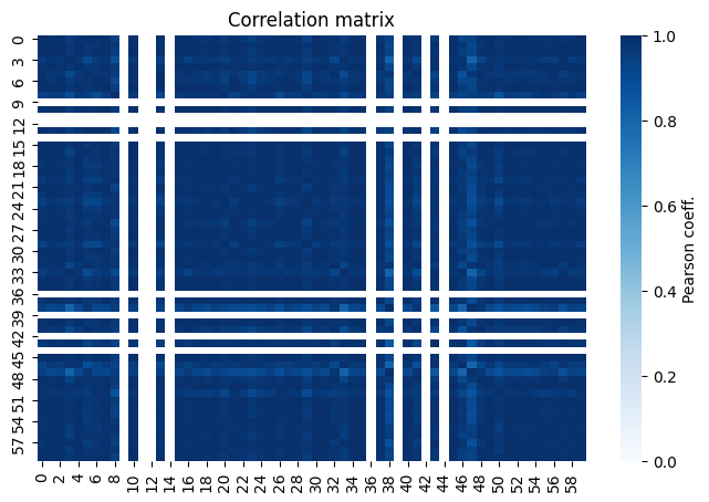
The empty rows and columns corresponds to bins with low statistics or zero expectation values in the fit variables. In our case, this comes from the signal template as can be seen in the plots at the begining of this notebook.
Visualize how many of eigenvariations are important#
[13]:
from sysvar import plot_cov_diff
fig, ax= plot_cov_diff(egd, save=False, filename = "test_figure")
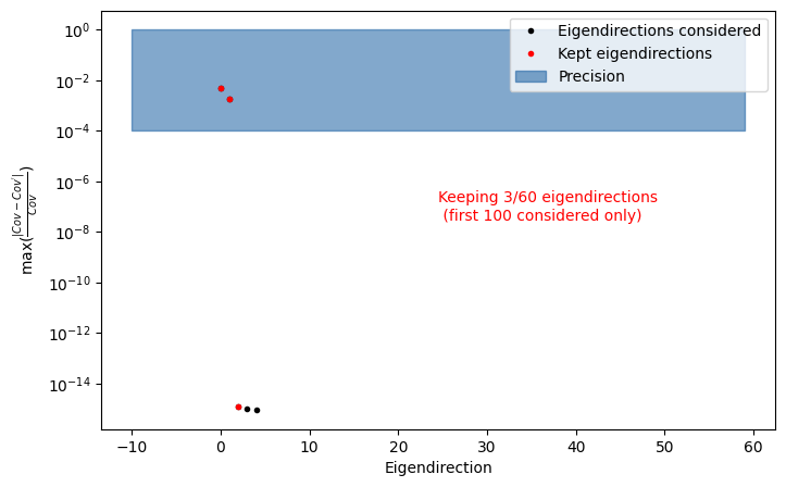
This truncation is only an initial estimate of how many eigenvariations are needed to preserve the analysis precision. By default, SysVar determines this by reconstructing the covariance matrix from the eigenvectors and comparing it to the original covariance. Eigenvectors are added one-by-one until the maximum element-wise normalised difference between the reconstructed covariance and the original becomes smaller than the precision (prc) specified by the user when calling
eigendecompose. This is still an approximation — and analysts must validate it for their own use case.
A more physics-oriented cross-check is to add the eigenvariations saved by SysVar as nuisance parameters in the fit one-by-one and monitor the uncertainty of the parameter of interest (e.g. on an Asimov dataset). When adding one more eigenvariation no longer changes the uncertainty, you have reached the number of relevant eigenvariations.
Note however: if you have already included all eigendirections saved by SysVar and the uncertainty on the parameter of interest still changes, then you should reduce the prc value (i.e. require a tighter precision) and repeat the eigendecomposition and validation.
The next sections detail the different types of corrections that SysVar provides, and how analysts can implement them in their analyses.